AItoday. AI ML DL Topics for the Day
AItoday : Temporary page for content of the day https://brahmavad.in/aitoday/
Go back to Main Reference page for all days https://brahmavad.in/iitkairef/
Date 20 June 2025 Friday EXAM Day Some Topics
Matrix
Transpose of Matrix
Matric Multiplication
Determinant
Inverse
Inner Product
Linear
2nd June, 2025
Lecture 1: Introduction to Artificial Intelligence (AI) Machine Learning (ML)
- • Overview of AI, ML
- • Regression
- • Classification
- • Supervised Learning
- • Unsupervised Learning
- • Deep Learning
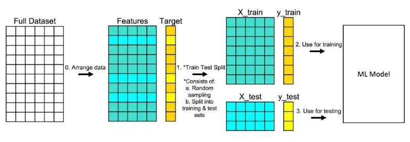
- • Test-Train Split
- • Metrics
- • Overview of AI, ML
- • Regression
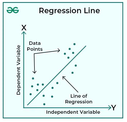
Regression is a statistical technique that relates a dependent variable to one or more independent variables. A regression model shows whether changes observed in the dependent variable are associated with changes in one or more of the independent variables.
- regression refers to a set of statistical processes used to estimate the relationships between a dependent variable (the one being predicted) and one or more independent variables (the predictors). It aims to model and predict the value of a continuous numerical variable based on other related variables.
Regression in Machine Learning:
- In machine learning, regression is a supervised learning task, meaning it learns from labeled data (input-output pairs).
- It’s used when the target variable (the dependent variable) is continuous, meaning it can take on any value within a range (e.g., house prices, stock prices, temperatures).
- Algorithms like linear regression, polynomial regression, and support vector regression are commonly used.
Key Concepts:
- Dependent Variable:The variable you are trying to predict or explain (e.g., house price).
- Independent Variables:The variables used to predict the dependent variable (e.g., house size, location).
- Regression Equation:The mathematical formula that describes the relationship between the variables.
- Regression Line/Curve:The visual representation of the relationship between variables on a graph.
Examples of Regression Applications:
- Financial Forecasting: Predicting stock prices, interest rates, or sales figures.
- Sales and Marketing: Estimating future sales based on advertising spend, seasonality, or promotions.
- Medical Research: Predicting patient outcomes based on various factors like age, gender, and medical history.
- Real Estate: Estimating house prices based on location, size, and other features.
Statistical Modeling:
- Regression analysis is a core statistical technique used to understand how changes in independent variables impact the dependent variable.
- The goal is to find a function that best fits the relationship between the variables, allowing for predictions of the dependent variable based on given values of the independent variables.
- Regression models can be linear, where the relationship is assumed to be a straight line, or non-linear, where more complex curves are used
- • Classification
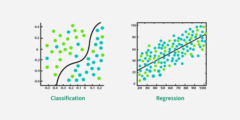
Classification and regression are both supervised machine learning tasks, but they differ in the type of output they predict. Classification predicts a discrete category or label, while regression predicts a continuous numerical value.
Classification:
- Goal: To categorize data points into predefined classes or labels.
- Output: Discrete, categorical values (e.g., “spam” or “not spam”, “cat” or “dog”).
- Examples: Email spam detection, image recognition, sentiment analysis.
- Algorithms: Logistic regression, support vector machines (SVM), decision trees, random forests.
Regression:
- Goal:To predict a continuous numerical value.
- Output:Continuous, numerical values (e.g., house price, stock price, temperature).
- Examples:Predicting house prices, stock price forecasting, predicting customer lifetime value.
- Algorithms:Linear regression, polynomial regression, support vector regression (SVR), decision trees.
In essence, classification helps you sort things into groups, while regression helps you predict a quantity
Is CNN classification or regression?
First, a classification-based CNN–LSTM is designed to perform multiclass damage detection tasks, and then a regression-based CNN–LSTM is developed for damage localization and severity prediction tasks.
- • Supervised Learning
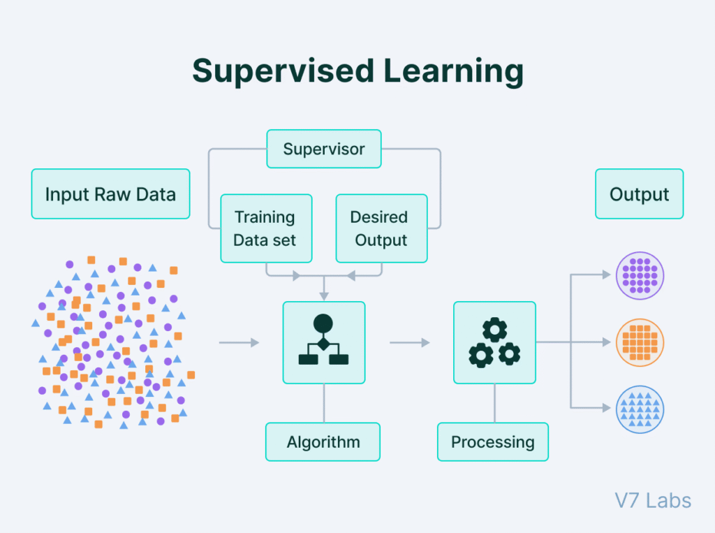
Supervised learning is a machine learning approach where an algorithm learns from a labeled dataset to make predictions or classifications. The algorithm learns the relationship between input data and their corresponding correct outputs, enabling it to predict outcomes for new, unseen data. Think of it as teaching a model with examples and their answers, so it can learn to predict the answers for new questions.
Here’s a more detailed explanation:
Key Characteristics:
- Labeled Data:Supervised learning relies on datasets where each input is paired with a correct output, or label.
- Training Process:The algorithm learns from this labeled data by identifying patterns and relationships between inputs and outputs.
- Prediction and Classification:The trained model can then be used to predict outcomes (regression) or assign categories (classification) to new, unlabeled data.
Examples:
- Spam Filtering:Training a model to identify spam emails by providing examples of spam and non-spam emails.
- Image Recognition:Training a model to identify objects in images by showing it labeled images of those objects.
- Medical Diagnosis:Training a model to predict diseases based on patient data and their diagnoses.
Types of Supervised Learning:
- Regression: Predicting continuous values, like house prices or stock prices.
- Classification: Categorizing data into predefined classes, like classifying emails as spam or not spam.
Benefits:
- Accurate Predictions: Labeled data allows for precise predictions and classifications.
- Pattern Recognition: Algorithms can identify complex patterns and relationships within the data.
- Task Automation: Supervised learning can automate tasks that would otherwise require human intervention.
In essence, supervised learning provides a powerful framework for building predictive models by leveraging labeled data to guide the learning process.
- • Unsupervised Learning
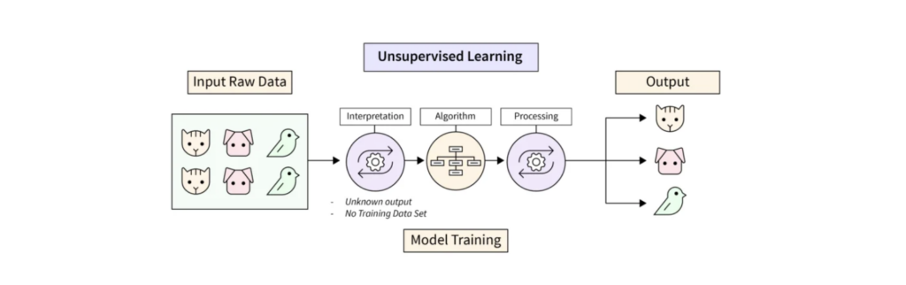
Unsupervised learning is a type of machine learning where algorithms learn from unlabeled data, discovering hidden patterns and structures without explicit guidance. Unlike supervised learning, it doesn’t rely on labeled examples or correct answers to guide the learning process. Instead, it explores the data to identify inherent groupings, relationships, or anomalies.
Here’s a more detailed explanation:
Key Characteristics:
- Unlabeled Data:The core feature of unsupervised learning is its use of data without pre-defined categories or labels.
- Pattern Discovery:Algorithms aim to find hidden patterns, structures, and relationships within the data.
- No Supervision:Unlike supervised learning, there’s no external “teacher” or labeled data to correct the algorithm’s outputs.
- Exploratory Analysis:Unsupervised learning is often used for exploratory data analysis, where the goal is to gain insights and understand the data’s characteristics.
- Clustering, Dimensionality Reduction, Anomaly Detection:Common tasks in unsupervised learning include clustering (grouping similar data points), dimensionality reduction (simplifying data by reducing the number of variables), and anomaly detection (identifying unusual data points).
Examples of Unsupervised Learning Applications:
- Customer Segmentation:Grouping customers based on purchasing behavior, demographics, or other characteristics.
- Anomaly Detection:Identifying fraudulent transactions, network intrusions, or unusual sensor readings.
- Recommendation Systems:Suggesting products or content based on user preferences and browsing history.
- Dimensionality Reduction:Reducing the number of features in a dataset while preserving important information.
- Image and Video Analysis:Discovering patterns and structures in visual data.
In essence, unsupervised learning is a powerful tool for exploring data, uncovering hidden structures, and gaining insights that might not be apparent through other methods.
Deep Learning
• Test-Train Split
•What is a test train split?
Train test split is a model validation procedure that splits a dataset into a training set and a testing set, which are used to determine how your model performs on new data.
- •
- • Test-Train Split
- • Metrics
REFERNCES : For Greater Details
https://www.appliedaicourse.com/blog/unsupervised-learning-in-machine-learning
https://builtin.com/data-science/train-test-split
3rd June, 2025
Lecture 3: Linear Regression for AIML
- • Regression Model
- • Multiple Regressors
- • Model Computation
- • Pseudo inverse
- • Online Learning
Lecture 3: Linear Regression for AIML
- • Regression Model
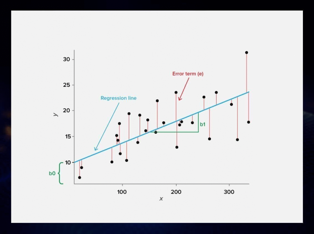
A regression model is a statistical tool that explores the relationship between a dependent variable and one or more independent variables. It aims to establish a mathematical function (a line or curve) that best describes this relationship, allowing for prediction and analysis of how changes in the independent variables affect the dependent variable.
Key aspects of regression models:
- Dependent Variable:The variable being predicted or whose relationship is being explored (also known as the response or target variable).
- Independent Variables:The variables that are used to predict or explain the dependent variable (also known as predictor variables).
- Relationship:Regression models aim to quantify the relationship between the dependent and independent variables, which can be linear or non-linear.
- Prediction:Once the model is established, it can be used to predict the value of the dependent variable for new, unseen data points.
- Analysis:Regression models can also be used to analyze the influence of each independent variable on the dependent variable, helping to understand which factors are most important.
Types of Regression Models:
- Linear Regression: Assumes a linear relationship between variables, represented by a straight line.
- Non-linear Regression: Models relationships that are not linear, using curves or other mathematical functions.
- Multiple Regression: Uses more than one independent variable to predict the dependent variable.
Examples:
- Predicting house prices based on size, location, and number of bedrooms (multiple linear regression).
- Modeling the relationship between advertising spending and sales revenue (simple linear regression).
- Forecasting future stock prices based on historical data (time series regression).
Representation of the regression model
The representation of a linear regression model is a linear equation.
Y=a+bX
- • Multiple Regressors
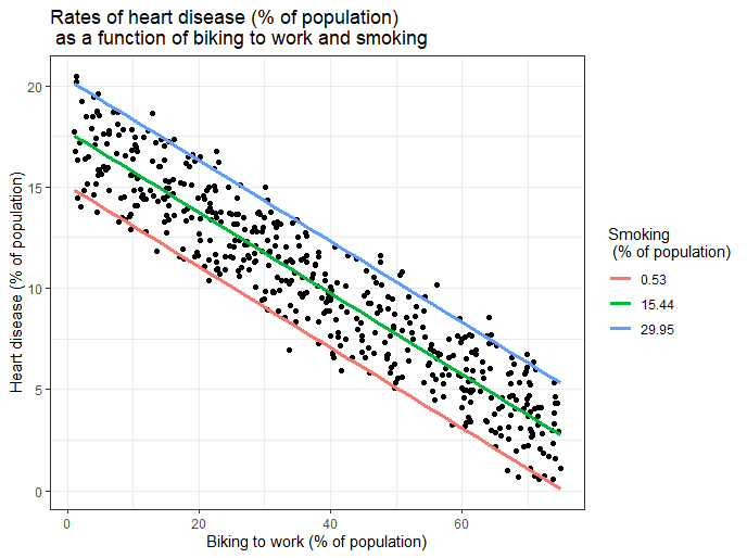
Multiple regression is a statistical technique that explores the relationship between one dependent variable and two or more independent variables. It aims to predict the value of a dependent variable based on the values of multiple independent variables. Essentially, it’s an extension of linear regression that incorporates more than one predictor variable.
Key Concepts:
- Dependent Variable:The variable being predicted or explained (also known as the outcome or response variable).
- Independent Variables:The variables used to predict the dependent variable (also known as predictor variables).
- Regression Coefficients:Values that indicate the strength and direction of the relationship between each independent variable and the dependent variable.
- Regression Equation:The equation that combines the independent variables and their coefficients to predict the dependent variable.
How it works:
- 1. Identify variables:Determine the dependent variable and the set of independent variables that might influence it.
- 2. Collect data:Gather data for all the variables involved in the analysis.
- 3. Apply the regression model:Use statistical software (like SPSS, R, Python, etc.) to fit the multiple regression model to the data.
- 4. Interpret the results:Analyze the regression coefficients, p-values, R-squared, and other statistics to understand the relationships between variables and the overall model fit.
Example:
Imagine trying to predict a student’s exam score (dependent variable). You could use multiple regression to see if revision time, test anxiety, lecture attendance, and gender (independent variables) all play a role in their performance.
Benefits of Multiple Regression:
- Predictive Power: Helps predict the value of a dependent variable based on multiple factors.
- Explanatory Power: Reveals which independent variables are most important in explaining the variation in the dependent variable.
- Control for Confounding Variables: Allows you to assess the unique contribution of each independent variable while controlling for the effects of other variables.
Different Types:
- Standard Multiple Regression: All independent variables are entered into the model simultaneously.
- Hierarchical Multiple Regression: Variables are entered into the model in a specific order, often based on theoretical considerations.
- Stepwise Multiple Regression: The software automatically selects the best set of independent variables for the model, often based on statistical criteria.
Assumptions:
Multiple regression relies on several assumptions about the data, including linearity, independence of errors, homoscedasticity, and normality. Violations of these assumptions can affect the validity of the results.
- • Model Computation
A model of computation is a framework that describes how a computer or a computational system functions. It defines the basic operations, memory, and communication mechanisms that a system can use. These models are crucial for understanding the capabilities and limitations of computation, and for designing and analyzing algorithms and systems.
Computational models play a crucial role in machine learning by providing a framework for understanding, simulating, and predicting the behavior of complex systems. They are used to represent real-world phenomena mathematically and computationally, allowing researchers to test hypotheses, analyze data, and develop intelligent systems. Machine learning algorithms then leverage these computational models to learn from data and make predictions or perform tasks.
Here’s a more detailed breakdown:
1. Representation and Simulation:
- Computational models translate real-world problems into mathematical and logical representations that can be processed by computers.
- These models can simulate the behavior of complex systems, such as the human brain, financial markets, or climate patterns, allowing researchers to explore various scenarios and understand underlying mechanisms.
- For example, in neuroscience, computational models are used to simulate neural networks and understand how information is processed in the brain.
2. Data Analysis and Pattern Recognition:
- Machine learning algorithms rely on computational models to learn from data and identify patterns.
- These models can be used to classify data, predict future outcomes, or discover hidden relationships within datasets.
- In the context of machine learning, computational models can be used to build predictive models for tasks like time series forecasting, image recognition, or natural language processing.
3. Model Validation and Refinement:
- Computational models can be used to test the validity of machine learning algorithms and identify areas for improvement.
- By comparing model predictions with real-world observations, researchers can refine the models and enhance their accuracy.
- This iterative process of model development and validation is crucial for building robust and reliable machine learning systems.
4. Examples in Different Fields:
- Neuroscience:Computational models are used to simulate neural networks, understand brain disorders, and develop new treatments.
- Finance:Models can simulate market behavior, assess risk, and develop trading strategies.
- Engineering:Models can simulate physical systems, optimize designs, and predict performance.
- Healthcare:Models can be used to personalize treatment plans, predict disease outbreaks, and develop new therapies.
In essence, computational models provide the foundation for machine learning by:
- Representing real-world phenomena in a computable form.
- Enabling the simulation and analysis of complex systems.
- Facilitating the development of intelligent systems that can learn from data.
- Allowing for the validation and refinement of machine learning algorithms.
- • Pseudo inverse
A pseudoinverse is a matrix inverse-like object that may be defined for a complex matrix, even if it is not necessarily square. For any given complex matrix, it is possible to define many possible pseudoinverses.
IN CONTEXT OF MACHINE LEARNING
In machine learning, the pseudoinverse (or Moore-Penrose pseudoinverse) of a matrix is a generalization of the matrix inverse that can be used even when the matrix is not square or is singular (i.e., has no regular inverse). It’s a crucial tool in various algorithms for solving linear systems, finding least-squares solutions, dimensionality reduction, and more.
Here’s how it’s used in machine learning:
1. Linear Regression:
- Linear regression aims to find the best-fitting line (or hyperplane in higher dimensions) to a set of data points.
- The pseudoinverse is used to calculate the coefficients (weights) of the regression equation that minimize the sum of squared errors, a process known as the least squares solution.
- If the matrix of input features has more rows (data points) than columns (features), it’s likely to be non-square. The pseudoinverse handles this scenario effectively, providing a solution even when a regular inverse doesn’t exist.
2. Dimensionality Reduction (PCA):
- Principal Component Analysis (PCA) is a technique to reduce the number of variables in a dataset while retaining most of the data’s variation.
- The pseudoinverse is involved in the calculation of the principal components, which are derived from the eigenvectors of the data’s covariance matrix.
3. Support Vector Machines (SVMs):
- SVMs are powerful classification algorithms. In some formulations, the pseudoinverse is used to calculate the optimal separating hyperplane.
4. Neural Networks:
- Certain neural network architectures, like Extreme Learning Machines (ELMs), utilize the pseudoinverse for faster training, especially in the output layer.
- The pseudoinverse can also be used to compute the weights in a neural network by solving a system of linear equations.
5. Solving Overdetermined and Underdetermined Systems:
- Overdetermined systems have more equations than unknowns, while underdetermined systems have more unknowns than equations. The pseudoinverse provides a way to find solutions (or approximate solutions) in both cases.
How it’s calculated:
- The pseudoinverse is often computed using the Singular Value Decomposition (SVD) of the matrix.
- SVD decomposes a matrix into three matrices, and the pseudoinverse is derived from these components.
In essence, the pseudoinverse is a versatile tool that allows machine learning algorithms to work effectively with various types of data and solve a wide range of problems, even when standard matrix inverses are not applicable.
GENERAL Idea
The pseudoinverse, also known as the Moore-Penrose inverse, is a generalization of the matrix inverse that extends to non-square and singular matrices. It’s a valuable tool for solving linear systems that may not have a unique solution or have no solution at all.
Here’s a more detailed explanation:
1. What is it?
- The pseudoinverse, denoted as A+, is a matrix that behaves like an inverse for matrices that don’t have a regular inverse (e.g., non-square or singular matrices).
- It satisfies the four Moore-Penrose conditions, which define its properties.
- The most common type of pseudoinverse is the Moore-Penrose pseudoinverse, which was independently described by E.H. Moore, Arne Bjerhammar, and Roger Penrose.
2. Why is it useful?
- Solving linear equations:It provides a “best fit” solution to linear systems that may be overdetermined (more equations than unknowns) or underdetermined (fewer equations than unknowns).
- Least squares solutions:In the case of overdetermined systems, the pseudoinverse finds the solution that minimizes the sum of squared errors (least squares solution).
- Singular matrices:It allows calculations with matrices that don’t have a standard inverse due to singularity.
- Applications:It’s widely used in various fields, including statistics (for linear regression), robotics (for inverse kinematics), and signal processing.
3. How is it calculated?
- The pseudoinverse is often calculated using the Singular Value Decomposition (SVD) of the matrix.
- SVD decomposes the matrix into three matrices, and the pseudoinverse is derived from these.
4. Key properties:
- For a square, invertible matrix, the pseudoinverse is equal to its regular inverse.
- It satisfies the four Moore-Penrose conditions.
- It provides a least-squares solution for overdetermined systems.
- It can be used to find solutions for underdetermined systems as well.
In essence, the pseudoinverse is a powerful tool that extends the concept of the matrix inverse to a wider range of scenarios, making it invaluable for solving linear systems and performing calculations where a regular inverse is not defined or doesn’t provide a meaningful solution.
- • Online Learning
- In machine learning, online learning is a dynamic approach where a model learns from a stream of data, updating its parameters with each new data point as it arrives. Unlike batch learning, which trains on the entire dataset at once, online learning allows for continuous adaptation to new information, making it suitable for real-time predictions and evolving datasets.
- Key characteristics of online learning:
- Sequential data:Data is processed one instance or a small batch at a time, rather than the entire dataset at once.
- Continuous updates:The model’s parameters are updated after processing each new data point, keeping the model current.
- Efficiency:Online learning can be computationally efficient, especially when dealing with large datasets or when resources are limited.
- Adaptability:The model continuously learns and adapts to changes in the data distribution, making it suitable for dynamic environments.
- Real-time predictions:Online learning enables the model to make predictions based on the most up-to-date information.
- Examples of online learning applications:
- Personalized recommendations:Recommender systems can continuously learn user preferences and update recommendations as new user data becomes available.
- Spam filtering:An email spam filter can learn to identify new spam patterns as they emerge, updating its model accordingly.
- Stock market prediction:Online learning can be used to predict stock prices based on real-time market data.
- Fraud detection:Models can be trained to detect fraudulent transactions by continuously learning from new transaction data.
- Adaptive website personalization:
- Websites can adapt content and layout based on user behavior and preferences as they browse.
In machine learning, online learning is a dynamic approach where a model learns from a stream of data, updating its parameters with each new data point as it arrives. Unlike batch learning, which trains on the entire dataset at once, online learning allows for continuous adaptation to new information, making it suitable for real-time predictions and evolving datasets.
Key characteristics of online learning:
- Sequential data:Data is processed one instance or a small batch at a time, rather than the entire dataset at once.
- Continuous updates:The model’s parameters are updated after processing each new data point, keeping the model current.
- Efficiency:Online learning can be computationally efficient, especially when dealing with large datasets or when resources are limited.
- Adaptability:The model continuously learns and adapts to changes in the data distribution, making it suitable for dynamic environments.
- Real-time predictions:Online learning enables the model to make predictions based on the most up-to-date information.
Examples of online learning applications:
- Personalized recommendations:Recommender systems can continuously learn user preferences and update recommendations as new user data becomes available.
- Spam filtering:An email spam filter can learn to identify new spam patterns as they emerge, updating its model accordingly.
- Stock market prediction:Online learning can be used to predict stock prices based on real-time market data.
- Fraud detection:Models can be trained to detect fraudulent transactions by continuously learning from new transaction data.
- Adaptive website personalization:Websites can adapt content and layout based on user behavior and preferences as they browse.
https://serokell.io/blog/regression-analysis-overview
https://www.scribbr.com/statistics/multiple-linear-regression
5th June, 2025
Lecture 4: Logistic Regression-Based AIML
- • Logistic Function
- • Class Probabilities
- • Likelihood and ML
- • Logistic Regression Metrics
- • Confusion Matrix
Logistic Regression-Based AIML
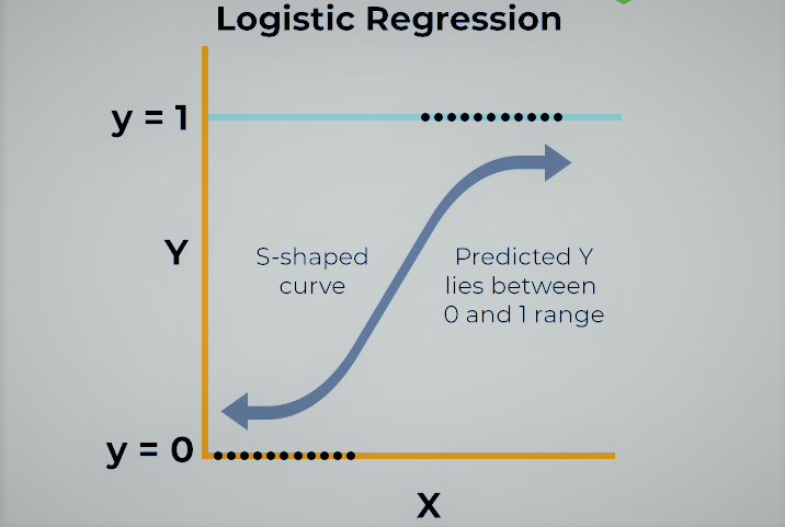
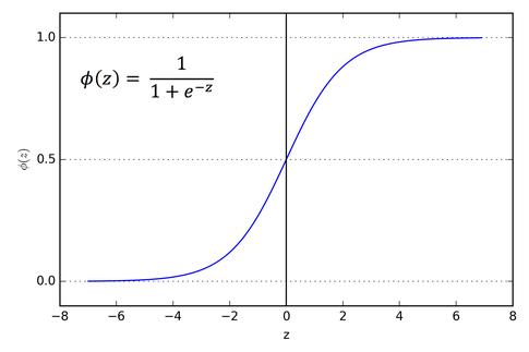
Logistic regression is a statistical method used for binary classification problems, where the goal is to predict the probability of a binary outcome (e.g., yes/no, true/false) based on input variables. Despite its name, it’s primarily used for classification, not regression. It models the log-odds of an event as a linear combination of the predictor variables.
Key Concepts:
- Binary Classification: Logistic regression deals with predicting one of two possible outcomes.
Log-odds:
It models the log of the odds of an event occurring, which is a linear function of the input variables.
Sigmoid Function:
The output of the linear model is transformed using the sigmoid function (also called the logistic function) to produce a probability between 0 and 1.
Supervised Learning:
It’s a supervised learning algorithm, meaning it learns from labeled data (data with known outcomes).
Linear Model:
While it’s a classification algorithm, it uses a linear model (similar to linear regression) to predict the log-odds.
How it works:
- 1. Linear Prediction: Logistic regression first calculates a weighted sum of the input features, similar to linear regression.
2. Sigmoid Transformation:
This linear output is then passed through a sigmoid function, which squashes the output to a range between 0 and 1, representing the probability of the event.
3. Classification:
A threshold (usually 0.5) is applied to this probability to make a binary prediction. If the probability is above the threshold, the outcome is classified as one class; otherwise, it’s classified as the other.
Assumptions:
- Binary Dependent Variable: The outcome variable must be binary (e.g., presence/absence of a disease).
Independence of Observations: Each observation should be independent of the others. No Perfect Multicollinearity: There should be no perfect correlation between the independent variables. Linearity of Log-odds: The log-odds of the outcome should be linearly related to the independent variables.
Applications:
- Medical Diagnosis: Predicting whether a patient has a disease or not.
Risk Assessment: Determining the likelihood of an event, like loan default. Spam Detection: Classifying emails as spam or not spam. Political Polling: Predicting whether a voter will support a particular candidate. Weather Forecasting: Predicting if it will snow or rain.
- • Logistic Function
A logistic function, also known as a sigmoid function, is a type of S-shaped curve that maps any input value to a value between 0 and 1. It’s commonly used in various fields like statistics, machine learning, and biology to model growth patterns that have a limited carrying capacity
- • Class Probabilities
In machine learning, class probabilities refer to the likelihood of an input belonging to a specific class. Instead of just predicting the most likely class, probabilistic models output a probability distribution across all possible classes, indicating how confident the model is in each classification. This approach is valuable for understanding uncertainty, making more informed decisions, and combining classifiers
- • Likelihood and ML
- • Logistic Regression Metrics
- • Confusion Matrix
https://www.linkedin.com/pulse/understanding-logistic-regression-model-laymans-words-omkar-sutar
https://www.linkedin.com/pulse/understanding-sigmoid-function-logistic-regression-piduguralla
6th June, 2025
Lecture 5: Support Vector Classifier (SVC) for Machine Learning
A support vector classifier is a type of machine learning model that can be used for classification tasks. Given a set of training examples, each labeled as belonging to one of two classes, the goal of the support vector classifier is to find a decision boundary that maximally separates the two classes.
- • SVM Structure
What is the SVM format?
A support vector machine (SVM) is a supervised machine learning algorithm that classifies data by finding an optimal line or hyperplane that maximizes the distance between each class in an N-dimensional space. SVMs were developed in the 1990s by Vladimir N
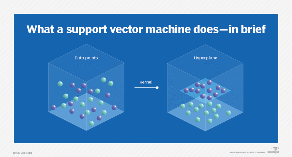
- • Maximum Margin Classifier
A maximum margin classifier, often used in Support Vector Machines (SVMs), aims to find the hyperplane (or decision boundary) that best separates two classes of data while maximizing the “margin” between them. The margin is the distance between the hyperplane and the nearest data points of either class.
Here’s a more detailed explanation:
Key Concepts:
- Hyperplane: A linear boundary that separates data points into different classes. In 2D, it’s a line, and in higher dimensions, it’s a hyperplane.
Margin:
The distance between the hyperplane and the closest data points of each class.
Support Vectors:
The data points that are closest to the hyperplane and determine the margin.
Objective:
The goal is to find the hyperplane that maximizes the margin while correctly classifying the data points.
How it works:
- 1. Finding the optimal hyperplane: The algorithm searches for the hyperplane that provides the largest possible margin.
2. Support Vectors:
The data points closest to the hyperplane are called support vectors. They play a crucial role in defining the margin.
3. Classification:
Once the optimal hyperplane is found, it is used to classify new, unseen data points.
Benefits:
- Robustness: A larger margin generally leads to better generalization and a more robust classifier.
Handles high-dimensional data:
SVMs, which utilize maximum margin classification, can effectively handle high-dimensional data.
Limitations:
- Computational cost: Training SVMs can be computationally expensive, especially for large datasets.
Sensitive to outliers: SVMs can be sensitive to outliers that influence the margin.
In summary, the maximum margin classifier seeks to find the best linear separation between data classes by maximizing the distance between the decision boundary and the nearest data points, leading to a robust and generalizable classification model.
- • Convexity and Convex Optimization
- • Kernel SVM
9th June, 2025
Lecture 6: Naïve Bayes Technique for AIML
- • Feature Vector
- • Likelihood and Prior Probabilities
- • Naïve Bayes Principle
- • Posterior Probability Evaluation
- • Gaussian Naïve Bayes
- • Movie Recommender System Example
10th June, 2025
Lecture 7: Discriminant Analysis (LDA) Based Data Classification
- • Gaussian Density
- • Multivariate Gaussian
- • Gaussian/ Linear Discriminant
- • Example Model Computation
12
: Data Clustering for Machine Learning
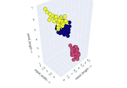
- • K-Means Algorithm
- • Centroid Computation
- • Cluster Assignment
- • Elbow Method for Number of Clusters
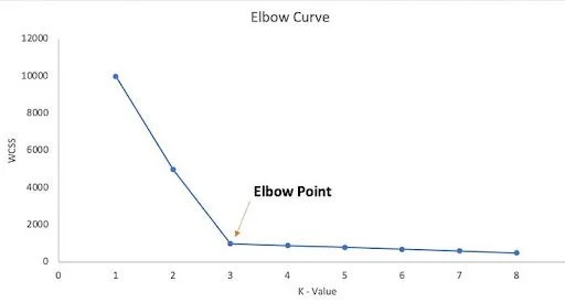
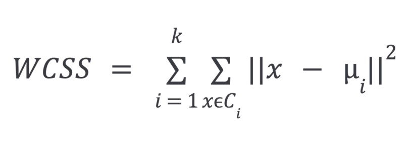
The Elbow Method is a heuristic used to find the optimal number of clusters (k) in K-Means clustering. It involves plotting the within-cluster sum of squares (WCSS) for different values of k and identifying the “elbow” point, where the rate of decrease in WCSS slows down significantly, indicating the optimal number of clusters.
Steps of the Elbow Method:
- Calculate WCSS: For a range of k values (e.g., 1 to 10), run the K-Means algorithm and calculate the WCSS for each k. WCSS measures the sum of squared distances between each data point and its cluster’s centroid.
Plot the results: Create a line graph with k on the x-axis and WCSS on the y-axis. Identify the elbow: The “elbow” point is the point on the graph where the decrease in WCSS starts to plateau, resembling an elbow shape. This point indicates the optimal number of clusters.
Interpretation:
- Before the elbow: Adding more clusters significantly reduces WCSS, indicating that the clusters are becoming more compact and the data points are closer to their respective centroids.
At the elbow:
The decrease in WCSS starts to slow down. Adding more clusters beyond this point doesn’t lead to a substantial improvement in the model’s fit.
After the elbow:
The reduction in WCSS becomes minimal, and the computational cost of adding more clusters may outweigh the benefits.
Example:
If the Elbow Method graph shows a clear elbow at k=3, it suggests that the optimal number of clusters for your K-Means clustering is 3.
- • Silhouette Score
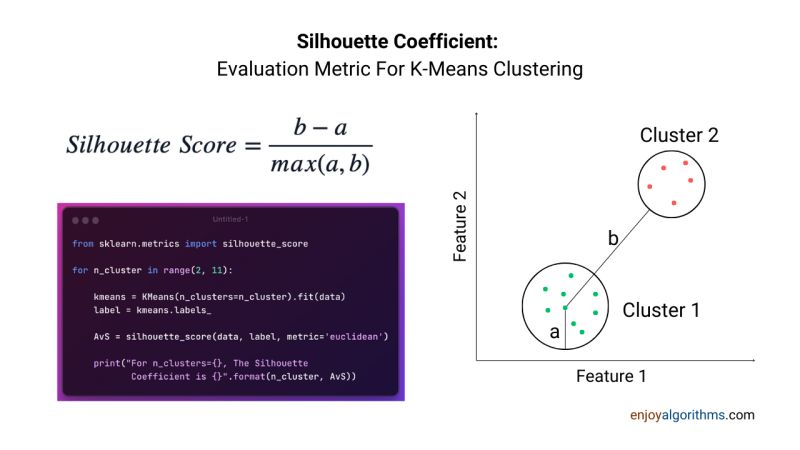
The Silhouette score is a metric used to assess the quality of clustering in data analysis. It measures how well each data point fits within its assigned cluster compared to other clusters, with values ranging from -1 to +1. A higher silhouette score indicates better-defined and more distinct clusters.
Understanding the Silhouette Score:
- Intra-cluster distance (a): For each data point, calculate the average distance to all other points within its cluster.
- Inter-cluster distance (b): For each data point, find the average distance to all points in the nearest neighboring cluster.
- Silhouette score calculation: For each data point, the silhouette score is (b – a) / max(a, b).
- Overall score: The silhouette score for the entire dataset is the mean of the individual data point scores.
Interpretation of Silhouette Scores:
- +1: Indicates that the data point is well within its cluster and far away from neighboring clusters.
0:
Indicates that the data point is on or very close to the decision boundary between two clusters.
-1:
Indicates that the data point might have been assigned to the wrong cluster.
Key Applications:
- Evaluating clustering algorithm performance: The silhouette score helps determine how well a clustering algorithm is performing.
Selecting the optimal number of clusters (k): By calculating silhouette scores for different values of k (number of clusters), you can choose the k that yields the highest score. Identifying data anomalies: Outliers or misclassified data points may have low silhouette scores.
In essence, the silhouette score provides a way to assess the quality of clustering results by quantifying how well data points are grouped into distinct and cohesive clusters.
https://builtin.com/data-science/elbow-method
https://www.enjoyalgorithms.com/live-machine-learning-course
Prepare for Text on 26 June 2025
Decision Tree Classifier
13th June, 2025
Lecture 9:Decision Tree Classifiers (DTC) for AIML
- • Optimal Feature Selection
- • Entropy
- • Conditional Entropy
- • Information Gain
- • Computation for Practical Restaurant Reservation Example
Lecture 9:Decision Tree Classifiers (DTC) for AIML
- • Optimal Feature Selection
- • Entropy
- • Conditional Entropy
- • Information Gain
- • Computation for Practical Restaurant Reservation Example
====
16th June, 2025
Lecture 10: Introduction to Neural Networks (NNs)
- • Neuron Structure and Properties
- • ANN Model
- • Activation Functions
- • One Hot Encoding
- • Categorical Crossentropy
| 16th June, 2025 | |
| 06:00 PM – 7:30 PM | Lecture 10: Introduction to Neural Networks (NNs) • Neuron Structure and Properties • ANN Model • Activation Functions • One Hot Encoding • Categorical Crossentropy |
17th June, 2025
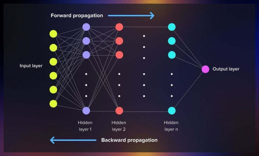
Leture 11: Deep Learning and Deep Neural Nets
- • Multi-layer Neural Networks
- • DNN Models
- • Dense and Sequential Architectures
- • NN Notation
- • Multi-layer Neural Nets
- • Gradient Descent
- • Backpropagation
- • Dropout Layers
| 17th June, 2025 | |
| 06:00 PM – 7:30 PM | Leture 11: Deep Learning and Deep Neural Nets • Multi-layer Neural Networks • DNN Models • Dense and Sequential Architectures • NN Notation • Multi-layer Neural Nets • Gradient Descent • Backpropagation • Dropout Layers |
19th June, 2025
Lecture 12: Convolutional Neural Networks (CNNs)
CNN Architectures • Convolution • Dot Product, • Padding • Hierarchical Structure • Max/ Average Pooling
| 19th June, 2025 | |
| 06:00 PM – 7:30 PM | Lecture 12: Convolutional Neural Networks (CNNs) • CNN Architectures • Convolution • Dot Product, • Padding • Hierarchical Structure • Max/ Average Pooling |
20th June, 2025
Project 12: Neural Network for analysis of Mobile Prices Dataset
- • Dataset Features
- • One Hot Encoding
- • Data Scaling
- • NN Model
- • Crossentropy
- • Adam Optimizer
- • Plots of Loss and Accuracy
20th June, 2025
06:00 PM – 7:30 PM
Project 12: Neural Network for analysis of Mobile Prices Dataset • Dataset Features
• One Hot Encoding
• Data Scaling
• NN Model
• Crossentropy
• Adam Optimizer
• Plots of Loss and Accuracy
| 20th June, 2025 | |
| 06:00 PM – 7:30 PM | Project 12: Neural Network for analysis of Mobile Prices Dataset • Dataset Features • One Hot Encoding • Data Scaling • NN Model • Crossentropy • Adam Optimizer • Plots of Loss and Accurac |
——–==========—
| 1st June , 2025 | |
| 12:00 PM – 12:30 PM | Zoom Test Session |
| Week-1 | |
| 2nd June, 2025 | |
| 06:00 PM – 7:30 PM | Lecture 1: Introduction to Artificial Intelligence (AI) Machine Learning (ML) • Overview of AI, ML • Regression • Classification • Supervised Learning • Unsupervised Learning • Deep Learning • Test-Train Split • Metrics |
| 7:30 PM-8:00 PM | Break |
| 8:00 PM – 9:15 PM | Lecture 2: Linear Algebra for AIML • Vector Representation • Inner Product • Orthogonality • Matrices • Matrix Inversion |
| 3rd June, 2025 | |
| 6:00 PM – 7:30 PM | Lecture 3: Linear Regression for AIML • Regression Model • Multiple Regressors • Model Computation • Pseudo inverse • Online Learning |
| 7:30 PM-8:00 PM | Break |
| 8:00 PM – 9:15 PM | Project 1: IRIS Dataset Regression using PYTHON • IRIS Dataset Features • Linear Regression Module • Mean Squared Error (MSE) • R2 Score |
| 4th June, 2025 |
| 4th June, 2025 | |
| Break Day |
| 5th June, 2025 | |
| 06:00 PM – 07:30 PM | Lecture 4: Logistic Regression-Based AIML • Logistic Function • Class Probabilities • Likelihood and ML • Logistic Regression Metrics • Confusion Matrix |
| 7:30 PM-8:00 PM | Break |
| 8:00 PM – 9:15 PM | Project 2: Boston Housing Price Analysis using PYTHON-Based Regression • Boston Housing set Features • Model Fitting • Model Performance • MSE, R2 Score • Regression Plot |
| 6th June, 2025 | |
| 06:00 PM – 7:30 PM | Lecture 5: Support Vector Classifier (SVC) for Machine Learning • SVM Structure • Maximum Margin Classifier • Convexity and Convex Optimization • Kernel SVM |
| 7:30 PM-8:00 PM | Break |
| 8:00 PM – 9:15 PM | Project 3: SCIKIT Package for Logistic Regression using Purchase/ Shopping Data • Purchase/ Shopping Dataset Features • Logistic Model Fitting • Confusion Matrix Display • Accuracy Score |
| Week-2 | |
| 9th June, 2025 | |
| 06:00 PM – 7:30 PM | Lecture 6: Naïve Bayes Technique for AIML • Feature Vector • Likelihood and Prior Probabilities • Naïve Bayes Principle • Posterior Probability Evaluation • Gaussian Naïve Bayes • Movie Recommender System Example |
| 7:30 PM-8:00 PM | Break |
| 8:00 PM – 9:15 PM | Project 4: IRIS Data Set classification using PYTHON-Based SVC • Dataset Features • Accuracy Metrics • Performance Evaluation |
| 10th June, 2025 | |
| 06:00 PM – 7:30 PM | Lecture 7: Discriminant Analysis (LDA) Based Data Classification • Gaussian Density • Multivariate Gaussian • Gaussian/ Linear Discriminant • Example Model Computation |
| 7:30 PM-8:00 PM | Break |
| 8:00 PM – 9:15 PM | Project 5: Breast Cancer Dataset Analysis using SVC • Breast Cancer Dataset Features • SVM Fit • Gaussian Kernel • Polynomial Kernel • Sigmoid Kernel • Performance Assessment Project 6: Naïve Bayes Classification of Purchase Dataset • Purchase Dataset Features • Gaussian NB Model Fitting • Accuracy Metrics • Confusion Matrix Display |
| 11th June, 2025 | |
| Break Day |
| 12th June, 2025 | |
| 06:00 PM – 7:30 PM | Lecture 8: Data Clustering for Machine Learning • K-Means Algorithm • Centroid Computation • Cluster Assignment • Elbow Method for Number of Clusters • Silhouette Score |
| 7:30 PM-8:00 PM | Break |
| 8:00 PM – 09:15 PM | No Session |
NOT in scope of Exam Today
| 13th June, 2025 | |
| 06:00 PM – 7:30 PM | Lecture 9:Decision Tree Classifiers (DTC) for AIML • Optimal Feature Selection • Entropy • Conditional Entropy • Information Gain • Computation for Practical Restaurant Reservation Example |
| 7:30 PM-8:00 PM | Break |
| 8:00 PM – 09:15 PM | Project 7: Discriminant Based Data Classification using IRIS Data Set • IRIS Dataset Features • LDA Model Fitting • Performance VisualizationProject 8: PYTHON Project for Data Clustering • K-Means Implementation • Elbow Curve • Silhouette Plot • Cluster Visualization |
| Week-3 | |
| 16th June, 2025 | |
| 06:00 PM – 7:30 PM | Lecture 10: Introduction to Neural Networks (NNs) • Neuron Structure and Properties • ANN Model • Activation Functions • One Hot Encoding • Categorical Crossentropy |
| 7:30 PM-8:00 PM | Break |
| 8:00 PM – 9:15 PM | Project 9: Building a DTC for IRIS Dataset using PYTHON • IRIS Dataset Features • DTC Model Fitting • Accuracy Score • Confusion Matrix Project 10: Decision Tree Classifier using for Purchase Logistic Data Set • Purchase Dataset Features • DTC Visualization • DTC Prediction • Performance Metrics |
| 17th June, 2025 | |
| 06:00 PM – 7:30 PM | Leture 11: Deep Learning and Deep Neural Nets • Multi-layer Neural Networks • DNN Models • Dense and Sequential Architectures • NN Notation • Multi-layer Neural Nets • Gradient Descent • Backpropagation • Dropout Layers |
| 7:30 PM-8:00 PM | Break |
| 8:00 PM – 9:15 PM | Distinguished Guest Lecture I: Dr. Dhananjay Ram, Senior Applied Scientist Amazon Web Services (AWS), Novel Architectures for LLM Bellevue, Washington, United States |
| 18th June, 2025 | |
| Break Day |
| 19th June, 2025 | |
| 06:00 PM – 7:30 PM | Lecture 12: Convolutional Neural Networks (CNNs) • CNN Architectures • Convolution • Dot Product, • Padding • Hierarchical Structure • Max/ Average Pooling |
| 7:30 PM-8:00 PM | Break |
| 8:00 PM – 9:15 PM | Project 11: PYTHON-based Neural Network using PYTHON for Boston Housing Dataset • Boston Dataset Features • Sequential NN Model • Model Fitting • Training Epochs • Accuracy Performance |
| 20th June, 2025 | |
| 06:00 PM – 7:30 PM | Project 12: Neural Network for analysis of Mobile Prices Dataset • Dataset Features • One Hot Encoding • Data Scaling • NN Model • Crossentropy • Adam Optimizer • Plots of Loss and Accuracy |
| 7:30 PM-8:00 PM | Break |
| 8:00 PM – 9:15 PM | Test prep 1:Test preparation 1 • Interview problem solving session • Solution discussion |
| Week-4 | |
| 23rd June, 2025 | |
| 06:00 PM – 7:30 PM | Distinguished Guest Lecture II: Dr. Karthikeyan Shanmugam, Research Scientist at Google DeepMind India (Bengaluru) |
| 7:30 PM-8:00 PM | Break |
| 8:00 PM – 9:15 PM | Project 13: Deep Learning for Fashion Classification using the MNIST Fashion Data Set • Fashion MNIST (Modified National Institute of Standards and Technology) Dataset Description • MNIST Dataset Features and Classes • CNN Modeling • CNN Training • Sparse Categorical Crossentropy • Loss/ Accuracy Plotting Project 14: Deep Learning for Digit Classification using MNIST Digit DataSet • MNIST Handwritten Digit Dataset Features • CNN Architecture • Data Encoding • Softmax Activation • Confusion Matrix • Plots of Loss and Accuracy |
| 24th June, 2025 | |
| Break Day | |
| 25th June, 2025 | |
| Break Day | |
| 26th June, 2025 | |
| 06:00 PM – 7:30 PM | Project 15: Deep Learning using the CIFAR Dataset • CIFAR-10 dataset (Canadian Institute for Advanced Research, 10 classes) • Dataset Visualization • CNN Architecture • Model Building and Compilation • Classification Accuracy • Confusion Matrix Metrics |
| 7:30 PM-8:00 PM | Break |
| 8:00 PM – 9:15 PM | Test prep 2: Test preparation 2 • Interview problem solving session • Solution discussion |
| 27th June, 2025 | |
| 06:00 PM – 07:30 PM | Distinguished Guest Lecture III: Dr. Bamdev Mishra, Principal Applied Scientist Microsoft India, Bangalore |
| 7:30 PM-8:00 PM | Break |
| 8:00 PM – 9:15 PM | Project 16: IMDB Dataset and Deep Learning for Movie Rating Classification • Internet Movie Database (IMDb) Dataset Description • Vectorization • Binary Crossentropy • Model Training • Training and Validation Accuracy Plots • Training and Validation Loss Plots |
Date 19 June 2025 Thursday
Convolutional Neural Networks (CNNs)
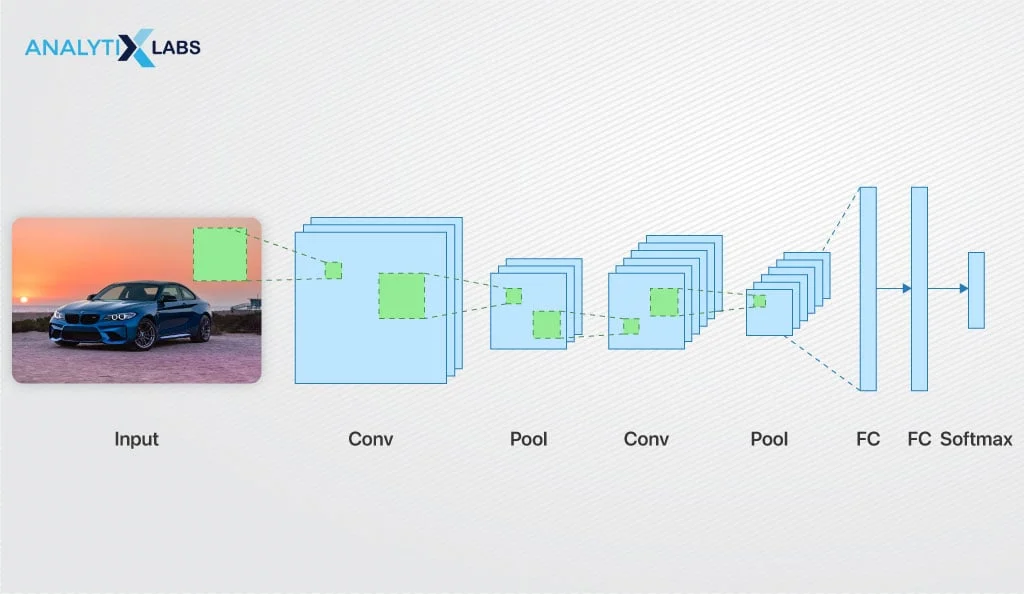
Convolutional Neural Networks
local receptive fields,
shared weights and biases, and
activation and pooling.
What are Convolutional Neural Networks (CNNs)?
CNN Architectures
HINDI VIDEO: What Is Convolutional Neural Network? Analytics India Guru Explains
Convoluted Layers
Pooling Layers
FC layers : Fully Connected Layers
CNN Architectures •
Convolution •
Dot Product, •
Padding •
Padding in Convolutional Neural Network
Learn With Jay
Hierarchical Structure •
Max/ Average Pooling
Max Pooling in Convolutional Neural Network
Understanding Different CNN Architectures
| 19th June, 2025 | |
| 06:00 PM – 7:30 PM | Lecture 12: Convolutional Neural Networks (CNNs) • CNN Architectures • Convolution • Dot Product, • Padding • Hierarchical Structure • Max/ Average Pooling |
| 7:30 PM-8:00 PM | Break |
| 8:00 PM – 9:15 PM | Project 11: PYTHON-based Neural Network using PYTHON for Boston Housing Dataset • Boston Dataset Features • Sequential NN Model • Model Fitting • Training Epochs • Accuracy Performance |
For Reference after June 2025 i.e when classes get over
Convolutional Neural Networks | CNN | Kernel | Stride | Padding | Pooling | Flatten | Formula
\
Convolutional Neural Network from Scratch | Mathematics & Python Code The Independent Code
https://www.analytixlabs.co.in/blog/convolutional-neural-network
https://www.analytixlabs.co.in/blog/convolutional-neural-network
Date 17 June 2025 Tuesday
Date 17 June
Topics for Today :
Leture 11: Deep Learning and Deep Neural Nets
- • Multi-layer Neural Networks
- • DNN Models
- • Dense and Sequential Architectures
- • NN Notation
- • Multi-layer Neural Nets
- • Gradient Descent
- • Backpropagation
- • Dropout Layers
Distinguished Guest Lecture I: Dr. Dhananjay Ram, Senior Applied Scientist Amazon Web Services (AWS), Novel Architectures for LLM Bellevue, Washington, United States
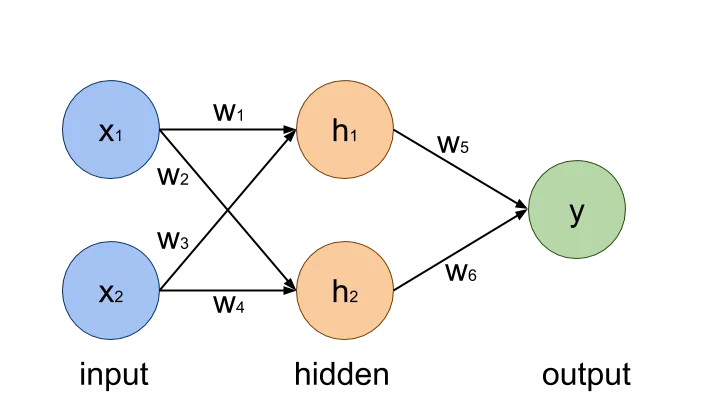
Multi-layer Neural Networks
DNN Models
Dense and Sequential Architectures
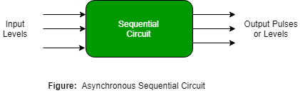
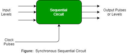
Types of Sequential Circuits
There are two types of sequential circuits
NN Notation
19-Notation for deep neural networks Dr.P.V.Yeswanth
https://cs230.stanford.edu/files/Notation.pdf

the equation represents how a vector y is computed from vector x, using matrix W, vector b and sigmoid function 𝜎.
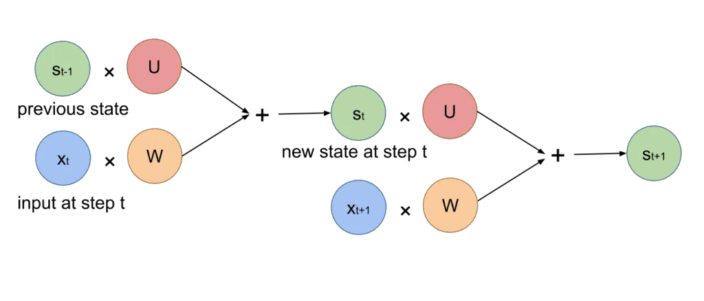
the well known Recurrent Neural Network (RNN), which is quite effective in learning patterns in sequences, is represented like this:

https://medium.com/@nityadav/neural-networks-mathematical-notation-9ef2a2badb3b
Multi-layer Neural Nets
Gradient Descent
Machine Learning Crash Course: Gradient Descent Google for Developers
Gradient Descent in 3 minutes Visually Explained
Backpropagation
What is Back Propagation IBM Technology 8 min
https://serokell.io/blog/understanding-backpropagation
Dropout Layers
Dropout layer in Neural Network | Dropout Explained | Quick Explained Developers Hutt
Novel Architectures for LLM